5 Steps to correctly prepare ,feature engineering and evaluate your data for your machine learning model

Stage 1: Collect and prepare data

The choice of data entirely depends on the problem you’re trying to solve.

Picking the right data must be your goal, luckily, almost every topic you can think of has several datasets which are public & free.3 of my favorite free awesome website for dataset hunting are:

Kaggle which is so organized. You’ll love how detailed their datasets are, they give you info on the features, data types, number of records. You can use their kernel too and you won’t have to download the dataset.
Reddit which is great for requesting the datasets you want.
Google Dataset Search which is still Beta, but it’s amazing.
UCI Machine Learning Repository, this one maintains 468 data sets as a service to the machine learning community.

The good thing is that data is means to an end, in other words, the quantity of the data is important but not as important as the quality of it. So, if you’d like to be independent and create your own dataset and begin with a couple of hundred lines and build up the rest as you’re going. That’ll work too. There’s a python library called Beautiful Soup.It is a library for pulling data out of HTML and XML files. It works with your favorite parser to provide idiomatic ways of navigating, searching and modifying the parse tree. It commonly saves programmers hours or days of work.

Data preparation may be one of the most difficult steps in any machine learning project.The reason is that each dataset is different and highly specific to the project. Nevertheless, there are enough commonalities across predictive modeling projects that we can define a loose sequence of steps and subtasks that you are likely to perform.This process provides a context in which we can consider the data preparation required for the project, informed both by the definition of the project performed before data preparation and the evaluation of machine learning algorithms performed after.

In this tutorial, you will discover how to consider data preparation as a step in a broader predictive modeling machine learning project.After completing this tutorial, you will know:

predictive modeling project with machine learning is different, but there are common steps performed on each project.
Data preparation involves best exposing the unknown underlying structure of the problem to learning algorithms.
The steps before and after data preparation in a project can inform what data preparation methods to apply, or at least explore.

Stage 2: Developing the idea

Once you’ve collected and prepared your data, you can distill business insights from it using ML applications. These applications may also allow you to do operational reporting, continuously observing real-time data as it’s generated. Use adaptive web applications to learn from user behavior and automatically optimize content for engagement, or build location-specific pricing models that reflect seasonal demand fluctuations.

Stage 3: Model Construction

While it is fun to think about all the tasks machine learning can do, it will be hard to figure out what is happening if your machine learning model is complicated. You must keep the first iteration of your model simple and focus on getting the infrastructure right. The first model provides the biggest boost to your product that is why it doesn't need to be fancy. But you will run into many more infrastructure issues than you expect. Before you expect to gain value from your machine learning models, you should determine:

Examples for your learning algorithm
What “good” and “bad” mean to your system
How to integrate your model into your application?

Choosing simple features will make it easier for you to ensure that:

The features reach your machine learning algorithm correctly
The features reach your model in the server correctly
The machine learning model learns reasonable weights

Once you have a system that does these three things correctly, it will provide you with baseline machine learning metrics and a baseline behavior that you can use to test more complex models.

Stage 4: Model Deployment

You should not expect that the model you are working on now will be the last one that you will launch. You should first consider whether the complexity you are adding in the first model is necessary. Many teams have launched machine learning models per quarter or more, for years. There are three basic reasons for launching new models:

You are developing new features
You are tuning and combining old features in new ways
You are tuning objectives.

For gaining value from your machine learning models, you have to know how to pair best algorithms with the right tools and processes. This will ensure that your models run as fast as possible, in huge enterprise environments.

Stage 5: Model evaluation

Overview

Evaluating a model is a core part of building an effective machine learning model
There are several evaluation metrics, like confusion matrix, cross-validation, AUC-ROC curve, etc.
Different evaluation metrics are used for different kinds of problems

I have seen plenty of analysts and aspiring data scientists not even bothering to check how robust their model is. Once they are finished building a model, they hurriedly map predicted values on unseen data. This is an incorrect approach.Simply building a predictive model is not your motive. It’s about creating and selecting a model which gives high accuracy on out of sample data. Hence, it is crucial to check the accuracy of your model prior to computing predicted values.

In our industry, we consider different kinds of metrics to evaluate our models. The choice of metric completely depends on the type of model and the implementation plan of the model.After you are finished building your model, these 11 metrics will help you in evaluating your model’s accuracy. Considering the rising popularity and importance of cross-validation, I’ve also mentioned its principles in this article.And if you’re starting out your machine learning journey, you should check out the comprehensive and popular ‘Applied Machine Learning’ course which covers this concept in a lot of detail along with the various algorithms and components of machine learning.

Confusion Matrix
F1 Score
AUC – ROC
Log Loss
Concordant – Discordant Ratio

1. Confusion Matrix

A confusion matrix is an N X N matrix, where N is the number of classes being predicted. For the problem in hand, we have N=2, and hence we get a 2 X 2 matrix. Here are a few definitions, you need to remember for a confusion matrix :

Accuracy : the proportion of the total number of predictions that were correct.
Positive Predictive Value or Precision : the proportion of positive cases that were correctly identified.
Negative Predictive Value : the proportion of negative cases that were correctly identified.
Sensitivity or Recall : the proportion of actual positive cases which are correctly identified.
Specificity : the proportion of actual negative cases which are correctly identified.

2. F1 Score

we are trying to get the best precision and recall at the same time? F1-Score is the harmonic mean of precision and recall values for a classification problem. The formula for F1-Score is as follows:

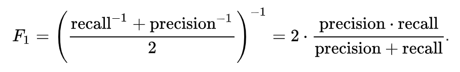
Now, an obvious question that comes to mind is why are taking a harmonic mean and not an arithmetic mean. This is because HM punishes extreme values more. Let us understand this with an example. We have a binary classification model with the following results:

Precision: 0, Recall: 1

Here, if we take the arithmetic mean, we get 0.5. It is clear that the above result comes from a dumb classifier which just ignores the input and just predicts one of the classes as output. Now, if we were to take HM, we will get 0 which is accurate as this model is useless for all purposes.

This seems simple. There are situations however for which a data scientist would like to give a percentage more importance/weight to either precision or recall. Altering the above expression a bit such that we can include an adjustable parameter beta for this purpose, we get:

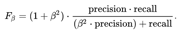
Fbeta measures the effectiveness of a model with respect to a user who attaches β times as much importance to recall as precision.

3. Area Under the ROC curve (AUC – ROC)

This is again one of the popular metrics used in the industry. The biggest advantage of using ROC curve is that it is independent of the change in proportion of responders. This statement will get clearer in the following sections.

Let’s first try to understand what is ROC (Receiver operating characteristic) curve. If we look at the confusion matrix below, we observe that for a probabilistic model, we get different value for each metric.

The ROC curve is the plot between sensitivity and (1- specificity). (1- specificity) is also known as false positive rate and sensitivity is also known as True Positive rate. Following is the ROC curve for the case in hand.

example of ROC curve

.90-1 = excellent (A)
.80-.90 = good (B)
.70-.80 = fair (C)
.60-.70 = poor (D)
.50-.60 = fail (F)

We see that the example fall under the excellent band for the current model. But this might simply be over-fitting. In such cases it becomes very important to to in-time and out-of-time validations.

4. Log Loss

AUC ROC considers the predicted probabilities for determining our model’s performance. However, there is an issue with AUC ROC, it only takes into account the order of probabilities and hence it does not take into account the model’s capability to predict higher probability for samples more likely to be positive. In that case, we could us the log loss which is nothing but negative average of the log of corrected predicted probabilities for each instance.

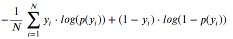
p(yi) is predicted probability of positive class
1-p(yi) is predicted probability of negative class
yi = 1 for positive class and 0 for negative class (actual values)

Let us calculate log loss for a few random values to get the gist of the above mathematical function:

Logloss(1, 0.1) = 2.303

Logloss(1, 0.5) = 0.693

Logloss(1, 0.9) = 0.105

If we plot this relationship, we will get a curve as follows:

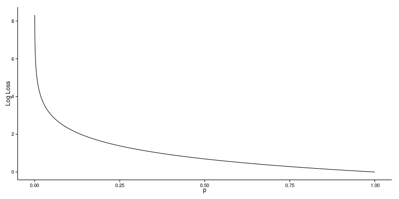
It’s apparent from the gentle downward slope towards the right that the Log Loss gradually declines as the predicted probability improves. Moving in the opposite direction though, the Log Loss ramps up very rapidly as the predicted probability approaches 0.

So, lower the log loss, better the model. However, there is no absolute measure on a good log loss and it is use-case/application dependent.

Whereas the AUC is computed with regards to binary classification with a varying decision threshold, log loss actually takes “certainty” of classification into account.

5. Concordant – Discordant ratio

This is again one of the most important metric for any classification predictions problem. To understand this let’s assume we have 3 students who have some likelihood to pass this year. Following are our predictions :

A – 0.9

B – 0.5

C – 0.3

Now picture this. if we were to fetch pairs of two from these three student, how many pairs will we have? We will have 3 pairs : AB , BC, CA. Now, after the year ends we saw that A and C passed this year while B failed. No, we choose all the pairs where we will find one responder and other non-responder. How many such pairs do we have?

We have two pairs AB and BC. Now for each of the 2 pairs, the concordant pair is where the probability of responder was higher than non-responder. Whereas discordant pair is where the vice-versa holds true. In case both the probabilities were equal, we say its a tie. Let’s see what happens in our case :

AB – Concordant

BC – Discordant

Hence, we have 50% of concordant cases in this example. Concordant ratio of more than 60% is considered to be a good model. This metric generally is not used when deciding how many customer to target etc. It is primarily used to access the model’s predictive power.

AI For Everyone

Search This Blog

Stages of ML development